Marching Squares - A Primer

In the world of computer graphics and game development, an algorithm that comes up often is Marching Squares. Quadtrees are also used often in the same fields, to optimize spatial queries. These two contents are fundamental for terrain generation, collision detection, and more.

This post focuses on understanding Marching Squares, and implementing it in JavaScript using p5.js. We’ll cover on optimizing this approach using Quadtrees in a follow up blog post.

But first, let’s build some motivation for why we need marching squares.

Motivation

Say we want to draw a mathematical function, for example, $y = sin(x)$. The most intuitive way of doing so, would be calculating the value of $y$ at each point, and connecting them with lines. Let’s take a look at this approach in the animation below:

You can play around with the function to see how it changes with frequency and resolution. Try doing the following things:

1. Decrease the resolution all the way down and see how it gets janky.
2. Max-out the resolution, and try increasing the frequency. You’ll notice how the function gets more hilly and complex.
3. Turn down both of them, and see how the function doesn’t even look close to the actual sin function.
4. Turn off the show lines option, and play around with the resolution. Notice how the number of points to each other as the resolution increases.
5. Turn on the show axes option, and repeat the steps above.

This changing of the graph is due to the changes in how we draw the function. As the resolution increases, we calculate and draw more and more points, in the same space. This makes the function look more accurate.

The Problem

We calculate the value of $y$, as per $y = sin(x)$ at each of these points. Then, we connect them all by lines which is the graph of the function.

Let’s take a look at the code for this approach.

// The equation we are trying to draw
const equation = x => sin(x)

// How often we'll be calculating the value of y
const resolution = 100
let points = []

function setup () {
  createCanvas(400, 225)

  // Caluclate the values of x, and y
  // and store them in the points array
  for (let i = 0; i < resolution; i++) {
    let x = (width / resolution) * i
    let y = (height / 2) * sin(2 * PI * (i / resolution))
    points.push(createVector(x, y))
  }
}

function draw() {
  background(220);
  translate(0, height / 2)

  // Connect each pair of points with a line
  for (let i = 0; i < points.length - 2; i++) {
    let p1 = points[i]
    let p2 = points[i + 1]
    line(p1.x, p1.y, p2.x, p2.y)
  }
}

You can install p5.js, and try out above code, or simply use the p5.js web editor.

This approach works well to a certain extent, however it has a very serious pitfall! Can you try to guess it? Here’s a hint - try to think about a function that gives two values of $y$ for any given $x$!

The Pitfall

It turns out that this approach does not work for implicit functions. Implicit functions are those that do not have a direct mapping between $x$ and $y$. Instead, they express a relationship between $x$ and $y$ in the form of an equation.

Consider the equation of a circle: $x^2 + y^2 = r^2$ where $r$ is the radius of the circle. Let’s try to draw this circle using the same approach as above.

// The equation we are trying to draw
const equation = x => sin(x) 
const r = 5
const equation = x => sqrt(r**2 - x**2) 

const resolution = 100
let points = []

function setup () {
  createCanvas(400, 225)

  for (let i = 0; i < resolution; i++) {
    let frac = i / resolution
    let x = width * frac
    let y = equation(x)
    points.push(createVector(x, y))
  }
}

function draw() {
  background(220);
  translate(0, height / 2)

  for (let i = 0; i < points.length - 2; i++) {
    let p1 = points[i]
    let p2 = points[i + 1]
    line(p1.x, p1.y, p2.x, p2.y)
  }
}

Replace the equation with the one above, and try running the code. You’ll notice that it doesn’t draw a circle, but instead a weird shape.

Contouring

Clearly, our simplistic approach is not enough to handle implicit functions. We need an algorithm, which can handle if a function outputs multiple values. However, thinking about it in an analytical way actually complicates the process. Let’s visualize the equation of a circle with the hopes of coming up with a better solution.

Consider the equation of a circle with radius = 5 units: $x^2 + y^2 = 25$. Let us superimpose a grid onto this circle. Our circle will be centered at the origin $O (0, 0)$.

You can try playing around with the radius of the circle - it’ll change in size as expected.

Now, turn on the Show Intersections checkbox to see where the grid lines intersect the circle and try changing the radius. If we focus solely on the squares with intersections, we start to notice some patterns. Do you see them? Try to focus on in what places the circle intersects with the squares of the grid. Sometimes the points of intersection are towards the right side of the square, and sometimes towards the left side. Sometimes, they are in the center.

Our goal is to plot this implicit curve, but as we saw in the previous $y = sin(x)$ example, computers don’t work very well with plotting continuous curves. So a crude, but simple approach to discretize the curve would be to turn it into a series of line segments. How about we evaluate each intersection square, and connect the two points where the circle intersects with the square?

You can see that the circle looks quite blocky, but it’s a good start. It’s certainly better than our previous approach. However, there is a caveat with this approach. As the radius of the circle reduces, the blockiness becomes more pronounced. This is because the circle is being approximated by a series of line segments, and the more segments we use, the more accurate the approximation becomes. Similarly, you can imagine that as we reduce the size of the squares (i.e. increase the resolution of the grid) the blockiness becomes less pronounced. From now on, we’ll be refering to these lines as contour lines.

While it’s not critical to our purpose, if you’re interested, here’s the code used to calculate these intersection lines. I encourage you to read it, since it’ll be beneficial in appraoching Marching Squares,

type Point = {
  x: number
  y: number
}

// Helper function to find intersections between a circle and a square
function findCircleSquareIntersections(
  circleCenter: Point,
  radius: number,
  squareTopLeft: Point,
  squareSize: number
): Point[] {
  const intersections: Point[] = []

  // Check each edge of the square for intersections with the circle

  // Bottom edge: y = squareTopLeft.y, x from squareTopLeft.x to squareTopLeft.x + squareSize
  findCircleLineIntersections(
    circleCenter,
    radius,
    { x: squareTopLeft.x, y: squareTopLeft.y },
    { x: squareTopLeft.x + squareSize, y: squareTopLeft.y },
    intersections
  )

  // Right edge: x = squareTopLeft.x + squareSize, y from squareTopLeft.y to squareTopLeft.y + squareSize
  findCircleLineIntersections(
    circleCenter,
    radius,
    { x: squareTopLeft.x + squareSize, y: squareTopLeft.y },
    { x: squareTopLeft.x + squareSize, y: squareTopLeft.y + squareSize },
    intersections
  )

  // Top edge: y = squareTopLeft.y + squareSize, x from squareTopLeft.x to squareTopLeft.x + squareSize
  findCircleLineIntersections(
    circleCenter,
    radius,
    { x: squareTopLeft.x, y: squareTopLeft.y + squareSize },
    { x: squareTopLeft.x + squareSize, y: squareTopLeft.y + squareSize },
    intersections
  )

  // Left edge: x = squareTopLeft.x, y from squareTopLeft.y to squareTopLeft.y + squareSize
  findCircleLineIntersections(
    circleCenter,
    radius,
    { x: squareTopLeft.x, y: squareTopLeft.y },
    { x: squareTopLeft.x, y: squareTopLeft.y + squareSize },
    intersections
  )

  return intersections
}

// Find intersections between a circle and a line segment
function findCircleLineIntersections(
  circleCenter: Point,
  radius: number,
  lineStart: Point,
  lineEnd: Point,
  intersections: Point[]
): void {
  // Convert line to parametric form: point = start + t * (end - start)
  const dx = lineEnd.x - lineStart.x
  const dy = lineEnd.y - lineStart.y

  // Solve quadratic equation for t at intersection points
  const a = dx * dx + dy * dy
  const b =
    2 *
    (dx * (lineStart.x - circleCenter.x) + dy * (lineStart.y - circleCenter.y))
  const c =
    (lineStart.x - circleCenter.x) * (lineStart.x - circleCenter.x) +
    (lineStart.y - circleCenter.y) * (lineStart.y - circleCenter.y) -
    radius * radius

  const discriminant = b * b - 4 * a * c

  if (discriminant < 0) {
    // No intersections
    return
  }

  // We have intersection(s)
  const t1 = (-b + Math.sqrt(discriminant)) / (2 * a)
  const t2 = (-b - Math.sqrt(discriminant)) / (2 * a)

  // Check if intersection point is on the line segment (t in [0, 1])
  if (t1 >= 0 && t1 <= 1) {
    intersections.push({
      x: lineStart.x + t1 * dx,
      y: lineStart.y + t1 * dy,
    })
  }

  if (t2 >= 0 && t2 <= 1) {
    intersections.push({
      x: lineStart.x + t2 * dx,
      y: lineStart.y + t2 * dy,
    })
  }
}

This approach finds all intersections squares (in $O(n^2)$ time) and checks all four edges of each intersection square, and calculates the intersection points ($O(1)$ time). It also requires special functions to calculate the intersections between a square and circle. Now imagine if we had some other graph, maybe a complicated curve like $x\times sin(x) + y \times sin(y) = 0$ - it would be a nightmare to make a function to calculate the intersections for that. This leads us to two critical questions, which will lead us to marching squares:

1. Is there a simpler way to find which grid squares intersect?
2. Can we identify a pattern to the lines which connect the intersection points?

Marching Squares

Now, we’re just two questions away from our goal. Let’s try to answer each one.

How to find intersections?

The approach we used in the previous section solved a quadratic equation to find the intersection points. This approach was specific to a circle, which means it won’t generalize well to more complicated/different graphs. Also, each graph would require a different method of calculating the intersection points - hence, this approach of mathematically computing intersection points is not viable.

Let us shed our pechant for calculating exact intersection points, and embrace some approximation. Let’s say we only want to find grid squares where the curve intersects the grid. This means that we will not consider:

1. Squares that are completely outside the curve.
2. Squares that are completely inside the curve.

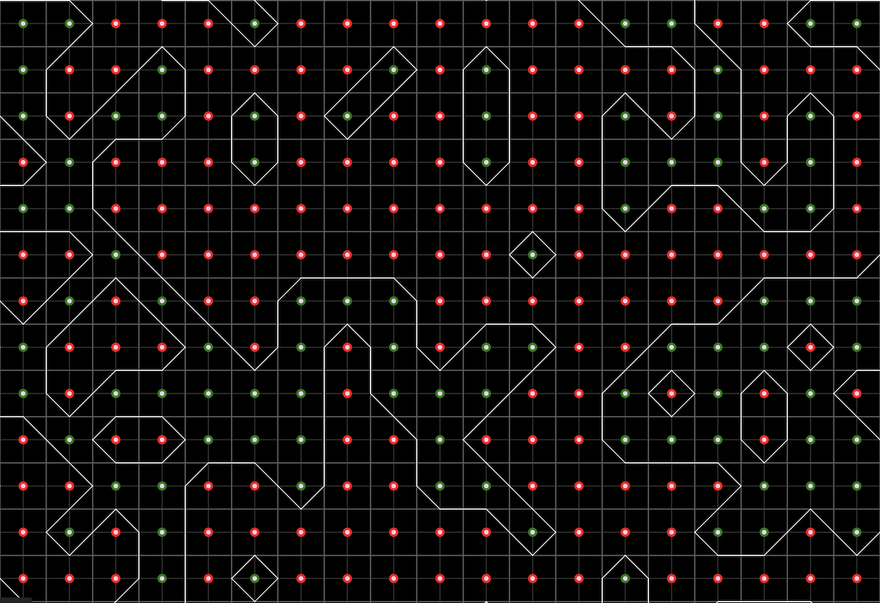
For the sake of exploration, let us assign a value of 1 to every point inside the curve, and a value of 0 to every point outside the curve. Let us mark these points accordingly.

To check whether the point is inside the circle, we can simply use this piece of code:

function isPointInsideCircle(
  point: Point,
  circleCenter: Point,
  circleRadius: number
): boolean {
  const distSq =
    (point.x - circleCenter.x) * (point.x - circleCenter.x) +
    (point.y - circleCenter.y) * (point.y - circleCenter.y)
  return distSq <= circleRadius * circleRadius
}

This calculates the distance of the given point from the center of the circle, and checks if it is less than or equal to the radius squared. However, this can be done in a generalized way for any function. Conside some implicit function of the form $f(x, y) = c$.

And we can mark every point as follows:

Now while we’ve been toying around with the math about contours for a bit, let’s take a more serious look at it. This process of marking 1’s and 0’s “inside” or “outside” is the process of creating a scalar field. The value at each point tells us whether that point is inside or outside our shape.

The boundary of our shape — in this case, is where the value transitions from 1 to 0. This boundary is called an isoline or contour line, and it represents all points where the function equals some constant value (like the radius of our circle).

This constant value can be anything. In the real world, it is often something like temperature, pressure or elevation. For example, here’s a map of contour lines representing elevation:

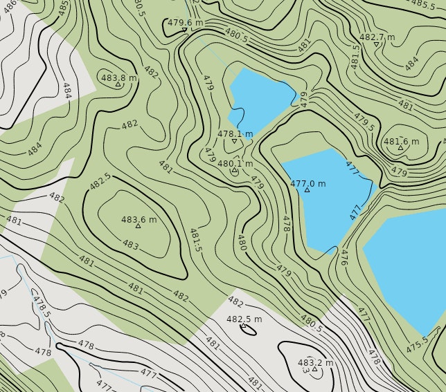
Everyline “isoline” in this image connects places with the exact same elevation. In the same way. The elevation at any particular isoline is called the isovalue. Take a look at the visualization below - it shows a circle at different isovalues.

In the general case, when we have a function $f(x, y) = c$, the constant c is called the isovalue. The isoline represents all the points where the function equals exactly this isovalue. For our circle example, the equation was $x^2 + y^2 = r^2$

Comparing this to $f(x, y) = c$, we can infer that

You might wonder about why we’re talking about this $c = 0$ value. It might not make much sense in 2D, but when we switch to 3D and we can see that $c$ represents the height of the surface at any given point. This is because the equation $f(x, y) = c$ describes a surface in 3D space, where $z = f(x, y)$. In the topographic map above, $c$ i.e. the elevation takes a continuous range of values.

Now, think back to when we were discussing marking values inside the circle with a $1$ and values outside the circle with a $0$. We did this to assign an isovalue to the contour created by the circle. This isovalue can be anything - however using $1$s and $0$s gives us another advantage in terms of representation - can you think what it is? Try thinking about how we can represent things using just $1$s and $0$s.

That’s right - it’s a binary representation. Now, we can cleanly define our intersections as follows:

1. Grid squares with all four corner values as $0$s lie completely outside the contour.
2. Grid squares with all four corner values as $1$s lie completely inside the contour.

This also means, that since the contour doesn’t pass through these squares, we can simply ignore them. Finally, we know that squares with mixed corner values must intersect the contour.

How to calculate contour lines?

Now that we’ve identified which grid squares intersect our contour line, we need to determine exactly how the contour passes through each of these squares. This is where the Marching Squares algorithm comes into play.

The key insight that the Marching Squares algorithm provides is a systematic way to determine how a contour line traverses through a grid square using the binary representation shennanigans we did before.

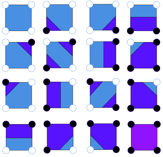
We assign each square a unique binary code based on the values of its four corners. We start from the bottom-left corner and move anticlockwise around the square, assigning a binary digit for each corner value. For example, a square with corners $(0, 0, 1, 1)$ would be assigned the binary code $0111$ i.e. $7$ in decimal. Since there are 4 corners, we geta 4 digit binary code - which means we assign numbers from 0 to 15 (i.e. a total of 16 cases).

Try playing around with this animation to get a feel for how this process works. You can see how the binary codes are assigned to each square using the All 16 Cases option from the dropdown. You can also explore Perlin Noise, Radial field and Wave field from the dropdown (remember - these are just different functions which leads to different scalar fields).

To have some more fun, click on the Custom option and draw your own scalar field! You’ll be able to see the binary values change in real time. Also, increase the resolution to see how the drawn curve looks smoother.

Alright, now let’s get back to the nitty-gritty of the algorithm. Hoepfully, you’ve got a good feel for how these contour lines are being calculated. Let’s make this notion of “calculating” contour lines a bit more concrete now.

Lookup Table

The Marching Squares algorithm provides us a lookup table - directly giving us the contour line for each of the 16 cases. This table is precomputed - which makes this approach much faster than the quadratic equation solving approach.

Let’s calculate the lookup table values for a couple of cases manually.

Case 0: All corners are outside (0000)

Case 1: Only bottom-left corner is inside (0001)

The contour line crosses the bottom edge somewhere between $(x_0, y_0)$ and $(x_1, y_0)$. With linear interpolation, the exact point depends on the actual values at these corners, but for our binary case, we can place it halfway:

Similarly, the contour crosses the left edge between $(x_0, y_0)$ and $(x_0, y_1)$:

The contour line for Case 1 connects these two points:

Case 5: The ambiguous case (0101)

Here, the bottom-left and top-right corners are inside (value 1), while the other two are outside (value 0). This creates an ambiguity: should the contour connect left-to-top or bottom-to-right?

As mentioned earlier, there are two possible ways to connect these points:

1. Connect left to top and bottom to right, making two contour lines:

2. Connect left to bottom and top to right, making two contour lines:

A similar ambiguity occurs with case $5 (0101)$. To resolve this ambiguity, there are quite a few ways - however they are out of scope of this blog post. Maybe I’ll cover them in a followup. But for now, let us say that we resolve this ambiguity in the simplest way i.e. to always connect diagonally opposite corners.

This approach is straightforward and efficient, but it may produce contour lines that don’t accurately represent the underlying data, especially if the true contour follows a different pattern.

Case 15: All corners are inside (1111)

Now that you have an idea of how we calculate the contours for these cases, here’s the complete lookup table.

And here’s a function which takes in the four corners of the grid square, and outputs the coordinates of the contour.

type Point = {
  x: number;
  y: number;
}

function marchingSquaresLookup(bottomLeft: Point, bottomRight: Point, topRight: Point, topLeft: Point, caseIndex: number): Point[] | Point[][] {
  // Calculate the midpoints of the edges
  const leftMid: Point = {
    x: bottomLeft.x,
    y: (bottomLeft.y + topLeft.y) / 2
  };
  const bottomMid: Point = {
    x: (bottomLeft.x + bottomRight.x) / 2,
    y: bottomLeft.y
  };
  const rightMid: Point = {
    x: bottomRight.x,
    y: (bottomRight.y + topRight.y) / 2
  };
  const topMid: Point = {
    x: (topLeft.x + topRight.x) / 2,
    y: topLeft.y
  };

  // Lookup table - returns array of points defining contour lines
  switch (caseIndex) {
    case 0: return []; // No contour (outside the shape)
    case 1: return [bottomMid, leftMid];
    case 2: return [bottomMid, rightMid];
    case 3: return [leftMid, rightMid];
    case 4: return [rightMid, topMid];
    case 5: return [[leftMid, topMid], [bottomMid, rightMid]] // ambiguous case
    case 6: return [bottomMid, topMid];
    case 7: return [leftMid, topMid];
    case 8: return [leftMid, topMid];
    case 9: return [bottomMid, topMid];
    case 10: return [[leftMid, bottomMid], [rightMid, topMid]]; // ambiguous case
    case 11: return [rightMid, topMid];
    case 12: return [leftMid, rightMid];
    case 13: return [bottomMid, rightMid];
    case 14: return [bottomMid, leftMid];
    case 15: return []; // no contour (inside the shape)
  }
}

Marching Squares!

Linear Interpolation

Alright, now this is the final piece of our desired algorithm. You might notice in the animation above that at lower resolutions, the contours look blocky. This is because we’re using assuming the curve contour passes through the midpoint of the edges of the square, however this might not be the case.

We need some way to find a realistic approximation of where the contour lies on the edge. One approach is to use linear interpolation between the edge points. Given two points $A$ and $B$ on the edge, and a value $t$ between 0 and 1 representing the position along the edge, we can calculate the interpolated point $P$ as follows:

Note that these points are 2D vectors, so this can also be written as

However for brevity, we’ll continue using the vector notation.

$t$ a.k.a parameter a.k.a. blend factor determines how far the interpolated point $P$ will be from A, and it uses some information from points $A$ and $B$ to do so. For our scalar field, $t$ is calculated based on the values of the scalar field at points $A$ and $B$.

Let’s consider the following variables:

Referring back to our equation of an implicit function $f(x, y) = c$, remember that $c$ is our isovalue. Hence,

Now, there can be five cases based on the values of $v_A$, $v_B$, and $v_{iso}$:

Case 1: $v_A = v_b$

If the scalar field values are equal, indicating that the isovalue passes through the midpoint of the edge connecting points A and B. Therefore,

Case 1: $v_A = v_iso$ or $v_B = v_iso$

If the above case is false, and one of the scalar field values is the same as the isovalue - this means that the contour will pass through one of the points $A$ or $B$. Therefore, the interpolated point $P$ will be either $A$ or $B$.

Case 3: $v_{iso} \in [v_A, v_B]$ or $v_{iso} \in [v_B, v_A]$

If above cases are false, and the isovalue is in the range of the two scalar values, then we must perform actual interpolation. In this case, the point $P$ lies somewhere between $A$ and $B$. We can calculate the position of $P$ using linear interpolation:

Finally, if $v_{iso} \notin [v_A, v_B]$ and $v_{iso} \notin [v_B, v_A]$, it means the contour won’t intersect with this edge at all, hence it can be safely ignored.

After all that math, let’s take a peek at the visualization of linear interpolation on a single grid square (for all edges)

Try playing around with the scalar field values and the isovalue. Try doing the following:

1. Setting both scalar values equal to each other
2. Setting one of the corner values equal to the isovalue
3. Setting the isovalue to be somewhere between the corner values
4. Setting the isovalue to be more than both the corner values

You’ll be able to see the math we discussed in action. Now, let’s implement this in Marching Squares to finally reach our goal.

We’re done! Yay!

Here’s the final p5.js sketch, which integrates linear interpolation with Marching Squares. You might have seen a similar animation like this previously in this article, but here it is again with linear interpolation (yes I’m very proud of it, thank you for noticing).

Yeah, that’s it - that’s Marching Squares! Here’s what the final implementation should look like. Try turning interpolation off - then on, you’ll see that the interpolated contour looks so much smoother than the non-interpolated one.

Conclusion

Advantages

1. Efficiency: Marching Squares is computationally efficient, using a precomputed lookup table to quickly determine contour patterns without complex mathematical calculations at runtime.

2. Simplicity: The algorithm is conceptually straightforward and relatively easy to implement, making it accessible even for those without extensive mathematical backgrounds.

3. Parallelizability: Each grid cell is processed independently, making the algorithm highly parallelizable and suitable for GPU implementation.

4. Resolution Control: By adjusting the grid resolution, you can control the trade-off between performance and contour detail.

Drawbacks

Despite its many advantages, Marching Squares does have several limitations:

1. Ambiguity Issues: As we’ve discussed, certain configurations (cases 5 and 10) are ambiguous and require additional resolution strategies, which can lead to inconsistencies if not handled properly.

2. Approximation Errors: Marching Squares produces an approximation of the true contour. For highly curved or intricate contours, this approximation may significantly deviate from the exact solution, especially with coarse grids.

3. Linear Interpolation Limitations: The algorithm typically uses linear interpolation to determine intersection points along grid edges, which can smooth out sharp features in the underlying data.

4. Topological Issues: In some cases, particularly with complex or rapidly changing scalar fields, Marching Squares might produce contours with incorrect topology, such as missing small features or creating spurious connections.

5. And more :(: For large datasets, memory overhead can be significant, and the algorithm may generate visual artifacts with inadequate grid resolution. Small features between grid points might be missed entirely, and boundary handling requires special care to avoid artifacts. Additionally, small changes in the isovalue parameter can dramatically alter the contour’s shape and topology.

Further Considerations

Quadtrees for Adaptive Resolution

One of the most effective optimization techniques is the use of quadtrees to create an adaptive grid:

Quadtrees recursively subdivide the domain into quarters, allowing for:

• Higher resolution in areas with complex contour behavior
• Lower resolution in areas with simple or no contours
• Significant reduction in the number of grid cells processed

The computational savings can be substantial, especially when contours occupy only a small portion of the domain. I originally planned to cover Quadtrees in this post, however seeing how long this one became, I decided to focus on the core algorithm and leave the advanced topics for future posts. I am currently working on a separate post dedicated to Quadtrees and their application in contour generation.

Multi-threading and Parallelization

The Marching Squares algorithm is inherently parallelizable since each grid cell can be processed independently:

• Divide the grid into sections and process each section on a different thread
• Use GPU acceleration via compute shaders for massive parallelism
• Implement a work-stealing pattern for load balancing when cell processing times vary

On modern hardware, parallel implementations can achieve order-of-magnitude speedups compared to sequential versions.

Marching Cubes (3D)

The natural extension of Marching Squares to 3D is the Marching Cubes algorithm, which generates isosurfaces (3D contours) from volumetric data:

• Each cube has 8 vertices, resulting in $2^8 = 256$ possible configurations
• These can be reduced to 15 base cases using symmetry
• The algorithm outputs triangles that form the isosurface mesh

It is used in Medical imaging (CT, MRI visualization), Visualization of 3D scalar fields (like Desmos), Games (for terrain generation) and more!

Dual Contouring

Dual Contouring improves upon traditional Marching Squares/Cubes by:

1. Generating vertices within cells rather than on edges
2. Preserving sharp features like corners and edges
3. Using Hermite data (function values and gradients)
4. Creating higher-quality contours with fewer elements

This approach produces contours that better preserve the features of the original scalar field, particularly when the field contains sharp transitions.

A word from me

And there you have it - that’s Marching Squares (well, at least the basics of it). When I learnt this algorithm, I had quite a rough journey understanding contours, isovalues and had to go through a lot of blog posts and videos (a lot of which you can find in the references).

All of this spurred from a sudden urge to make a Manim alternative which could completely work on the web - and this is how it turned out. Be that as it may, I hope you liked this post. This was my attempt at explaining Marching Squares, the way I’d have liked to learn it. Hopefully, you enjoyed it. Thanks for reading!