Image Processing Techniques in Python with OpenCV: Aruco Markers, Grayscaling, Binarization, and Contours

Obstacle Detection and Area Calculation from Overhead Drone Images using OpenCV

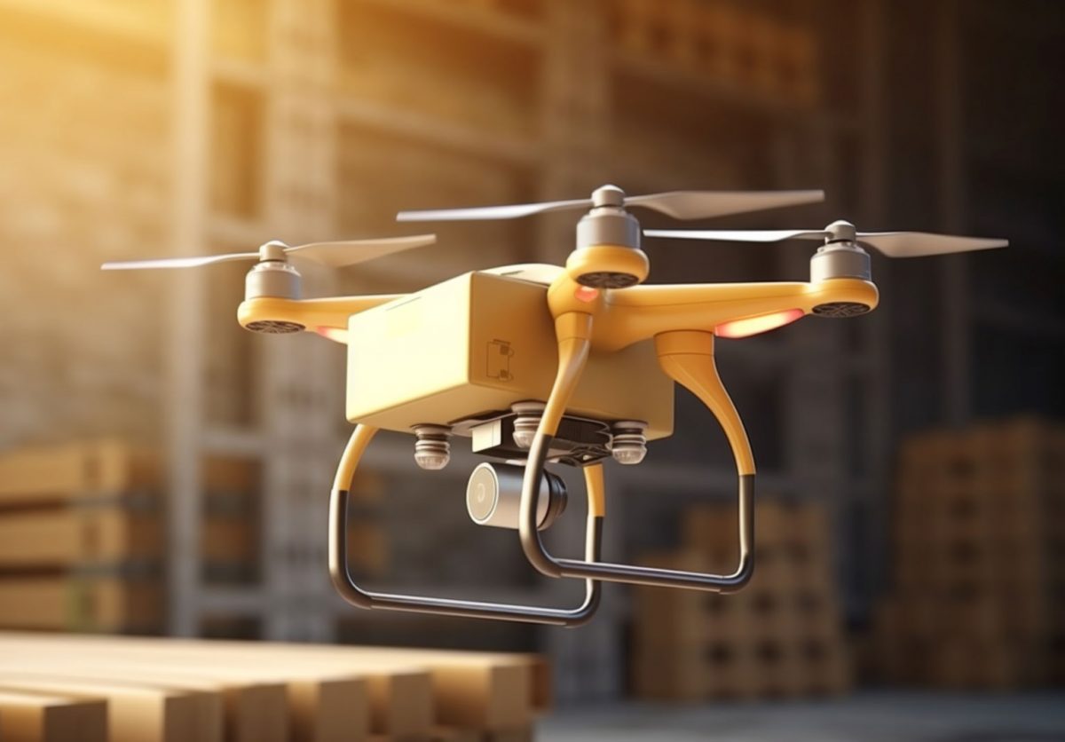
In the 2024 Eyantra Robotics Competition, we were tasked with developing a system to detect and analyze obstacles in overhead drone images. This involved us being provided with an image such as the one below, which shows the drone flying over a warehouse site.

We were tasked with detecting and analyzing the obstacles in the image. The process for the same involved image procesing techniques like

1. Grayscaling
2. Binarization
3. Aruco Marker Detection
4. Perspective Transformation
5. Contour Detection

Let us discuss each of these techniques, andd how we applied them in detail.

---

1. Grayscaling

1a. But before that, some preprocessing

The first step involves preprocessing the image slightly, to prepare it for further transformation. Firstly we read the given image (which was passed as an argument to the python script, but that is irrelevant to this post) andd resize it to a predetermined size (1000x1000) in this case.

image = cv2.imread(self.image_path) # Read the image
frame = cv2.resize(image.copy(), (self.width, self.height)) # Resize the image

1b. Now to the good stuff

Now, we convert the image to grayscale. OpenCV natively uses the BGR (blue-green-red) format instead of the conventional RGB that we are usedd to. Hence we must use cv2.COLOR_BGR2GRAY as a parameter.

# Convert the image from BGR to grayscale
frame = cv2.cvtColor(frame, cv2.COLOR_BGR2GRAY)

Under the hood of OpenCV, grayscaling works by multiplying each of the R, G and B components by a particular constant, which are then added in order to obtain a corresponding gray.

$Gray = 0.299 * R + 0.587 * G + 0.114 * B$

This is called a weighted sum. This is a simple yet effective method as it can be easily parallelized and runs very fast for individual pixels. One condition is that all the constants must add up to 1.

The $Gray$ value we obtain from the above equation is assigned to all three channels of the pixels. That means, for some BGR pixel $(255, 123, 45)$; we get

$Gray = 0.299 * 45 + 0.587 * 123 + 0.114 * 255 \newline \therefore Gray = 13.455 + 72.201 + 29.325 \newline \therefore Gray = 114.981 \approx 115$

Hence the output of the grayscaling process in our example will be a pixel with all channels set to 115, i.e. $(115, 115, 115)$.

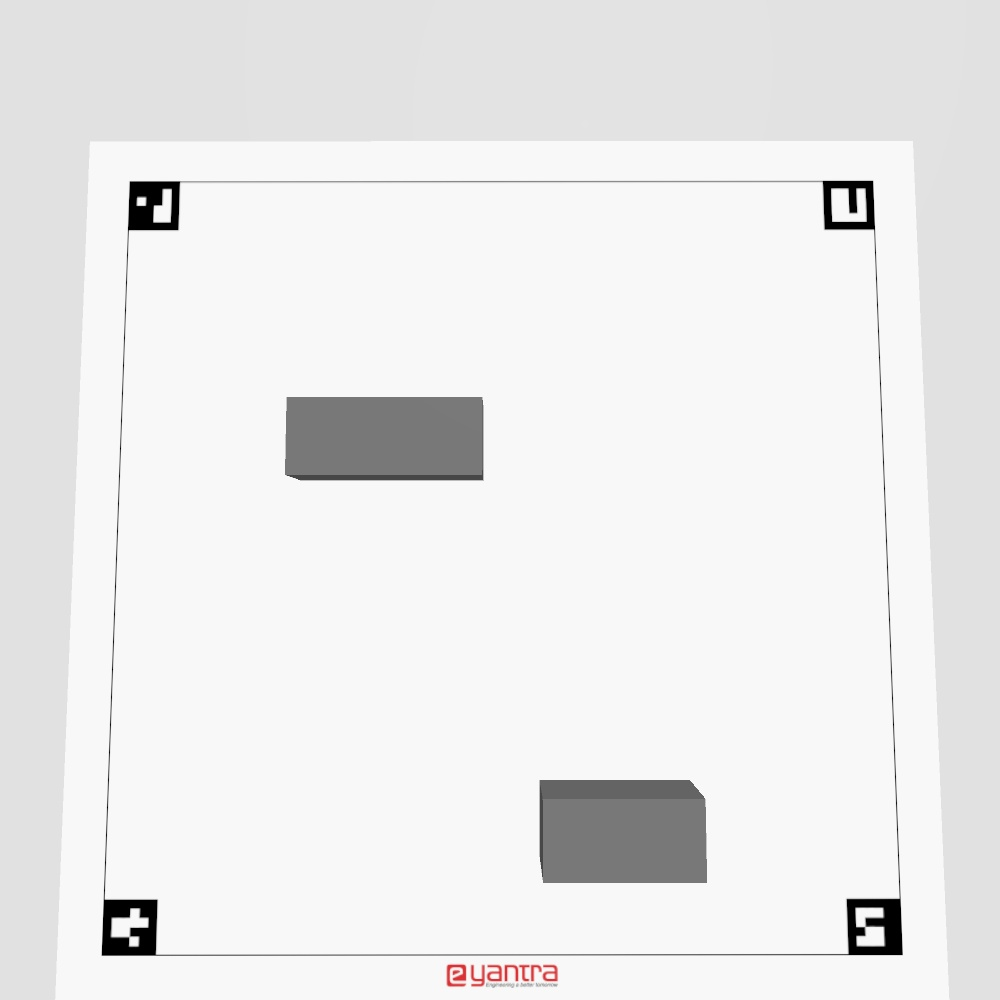
This exact process is applied to all pixels in the image which results in an image like the one shown below.

2. Binarization

Even though we grayscaled the image, from a computers perspective, it’s still quite difficult to parse. This is mainly because there are still a lot of colors, which makes it difficult to identify the Aruco markers we want to detect.

The solution to this is to binarize the image, which means to convert all the colors in the image to either black or white.

Now, there are multiple methods of binarizing an image. These include:

1. Global Thresholding
2. Adaptive Thresholding
3. Otsu’s Binarization
4. Guassian-based Otsu’s Binarization

Let us focus mainly on the first two, which are comparably simpler.

Global thresholding

It uses a single threshold value for the entire image. Every pixel is compared to this threshold, and based on this comparison, it is classified as either foreground (white) or background (black).

For a pixel value $I(x, y)$ at coordinates $(x, y)$:

$$B(x, y) = \begin{cases} 255 & \text{if } I(x, y) > T \\ 0 & \text{if } I(x, y) \leq T \end{cases}$$

Where:

• $T$ is the threshold value.
• $B(x, y)$ is the resulting binary image.
• Pixel values greater than $T$ are set to white (255), and those less than or equal to $T$ are set to black (0).

Global thresholding works well when the image has consistent lighting across the entire scene.

Adaptive thresholding

It calculates the threshold value dynamically for different regions of the image. Instead of using a single threshold for the whole image, the threshold is computed for small, localized neighborhoods of pixels. This makes it effective for images with varying lighting conditions.

For a pixel $I(x, y)$, the threshold $T(x, y)$ is calculated based on the intensity values of neighboring pixels in a window of size $W \times W$, typically using the mean or weighted mean.

1. Mean Adaptive Thresholding: $T(x, y) = \frac{1}{W \times W} \sum_{(i,j) \in W} I(i,j) - C$ Where:

• $W \times W$ is the size of the local region.
• $C$ is a constant that can be subtracted from the mean to adjust the threshold sensitivity.

2. Gaussian Adaptive Thresholding: $T(x, y) = \sum_{(i,j) \in W} G(i,j) \cdot I(i,j) - C$ Where:

• $G(i,j)$ is the Gaussian weight for the pixel at $(i,j)$ in the window.
• $C$ is a constant subtracted from the result.

Adaptive thresholding is ideal for images where lighting conditions vary, such as scanned documents or photos with shadows.

What we used

We decided to use simply global thresholding, since the top-view had consistent lighting. Moreover, while experimenting with found that the ddetection of Aruco markers would not work as effectively with adaptive thresholding methods like gaussian thresholding or otsu’s binarization.

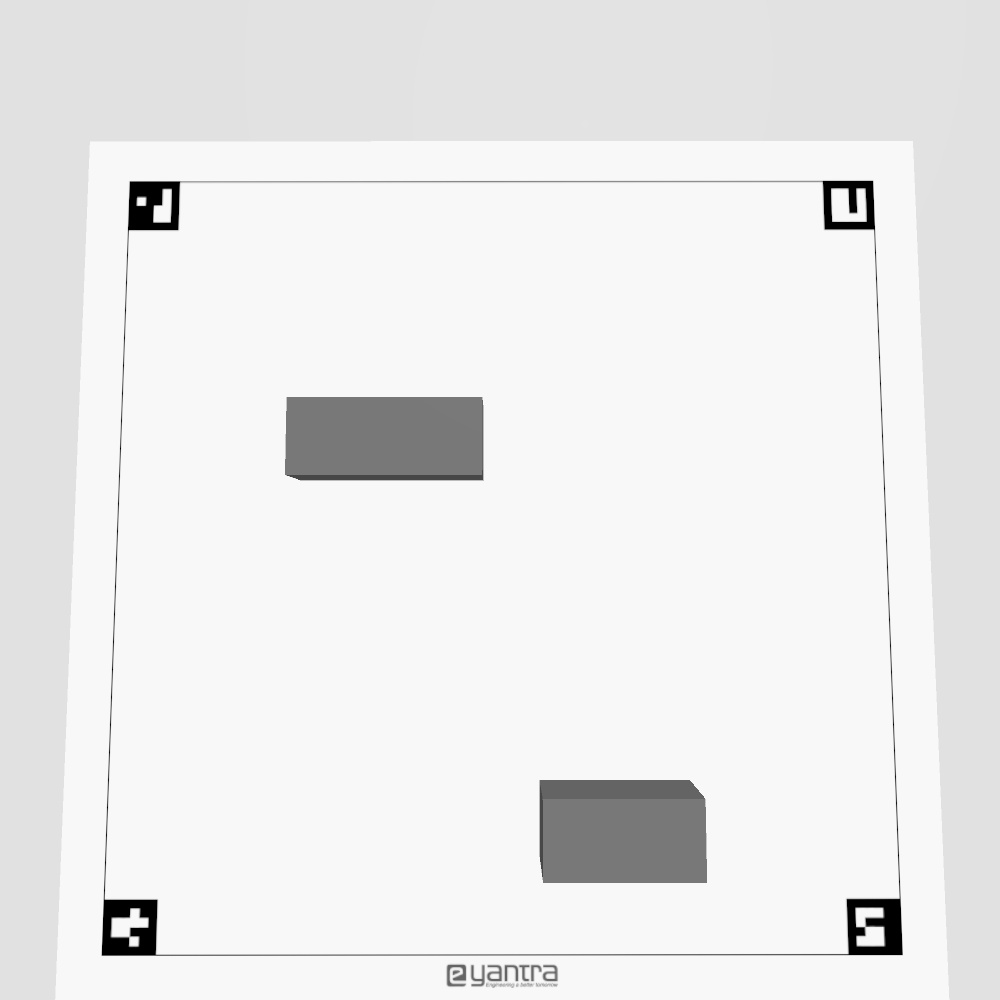
_, frame = cv2.threshold(frame, 70, 255, cv2.THRESH_BINARY)

Using the above code, we binarized the image, where any pixel with gray value less than 70 would become black and those with gray valu emore than 70 would become white. This value of 70, was found through trial and error to see which worked best with teh Aruco marker detection functions.

The binarization resulted in an image like the one shown below.

---

3. Aruco Marker Detection

What even is an Aruco marker?

A fiducial marker is a type of marker that is used in computer vision and robotics as a point of reference. These are easily identifable by a computer, and are used to identify end-points, edges, etc. of various objects from images.

Aruco markers are a type of fiducial marker system consisting of black-and-white, square-shaped patterns used in computer vision tasks for easy detection and identification. Each marker contains a unique binary pattern encoded in a grid, allowing it to be distinguished from others. The surrounding black border helps to detect the marker’s edges, while the internal grid is used to identify the specific marker ID. These markers are commonly used in robotics, augmented reality (AR), and camera calibration because they enable precise position and orientation tracking.

After the previous two steps, i.e. grayscaling and binarization, the Aruco markers are detected using the following process:

1. Contour Detection:

   • The algorithm then detects contours in the thresholded image using cv2.findContours(). Contours are continuous curves that define the boundaries of shapes, so this step identifies the outlines of quadrilateral shapes, which are likely Aruco markers.

2. Polygon Approximation:

   • For each contour, OpenCV applies a polygon approximation (cv2.approxPolyDP()), which simplifies the contour into a polygon with fewer vertices. The goal is to approximate the contour with four vertices (a quadrilateral), as this shape likely represents a marker.

3. Perspective Correction:

   • The detected quadrilaterals are then perspective-corrected to eliminate distortions due to the camera’s viewing angle. This step is crucial because markers viewed from different angles will appear distorted (trapezoidal instead of square). OpenCV uses homography transformation (cv2.getPerspectiveTransform()) to warp the detected marker into a standard square shape.

4. Marker Verification:

   • Once a quadrilateral is transformed into a square, the algorithm verifies whether it contains a valid Aruco marker by checking the black-and-white grid inside. The grid is compared against predefined marker dictionaries (such as DICT_4X4_50 or DICT_6X6_1000), which contain possible binary patterns.

5. Decoding:

   • After a valid marker is identified, the binary pattern inside the marker is decoded to extract the unique ID. This is done by reading the internal grid and interpreting the arrangement of black (0) and white (1) cells.

The above 5 steps are done using the cv2.aruco.detectMarkers() function, which is a part of the OpenCV library. This function takes an image, a marker dictionary, and optional parameters to detect and decode the markers.

parameters = aruco.DetectorParameters()
aruco_dict = cv2.aruco.getPredefinedDictionary(self.ARUCO_DICT)
corners, ids, rejectedImgPoints = aruco.detectMarkers(
  frame,
  aruco_dict,
  parameters=parameters
)

In the above code, we first, the dictionary which contains the pattern of Aruco markers present in the image is found through trial and error. The following snippet of code is used to find the correct dicitonary.

not_none_dicts = []
for name, aruco_dict_name in self.ARUCO_DICT.items():
    parameters = aruco.DetectorParameters_create()
    aruco_dict = cv2.aruco.Dictionary_get(aruco_dict_name)
    corners, ids, rejectedImgPoints = aruco.detectMarkers(
      frame, 
      aruco_dict, 
      parameters=parameters
    )
    # print(corners, ids, rejectedImgPoints)
    if ids is not None:
        not_none_dicts.append(name)

print(not_none_dicts)

The ahove code simply runs the marker detection for all available dictionaries and prints the IDs of thr markers detected. From looking at the image, we knew it contained 4 Aruco markers, so we picked the first dictionary which resulted in 4 markers being successfully detected.

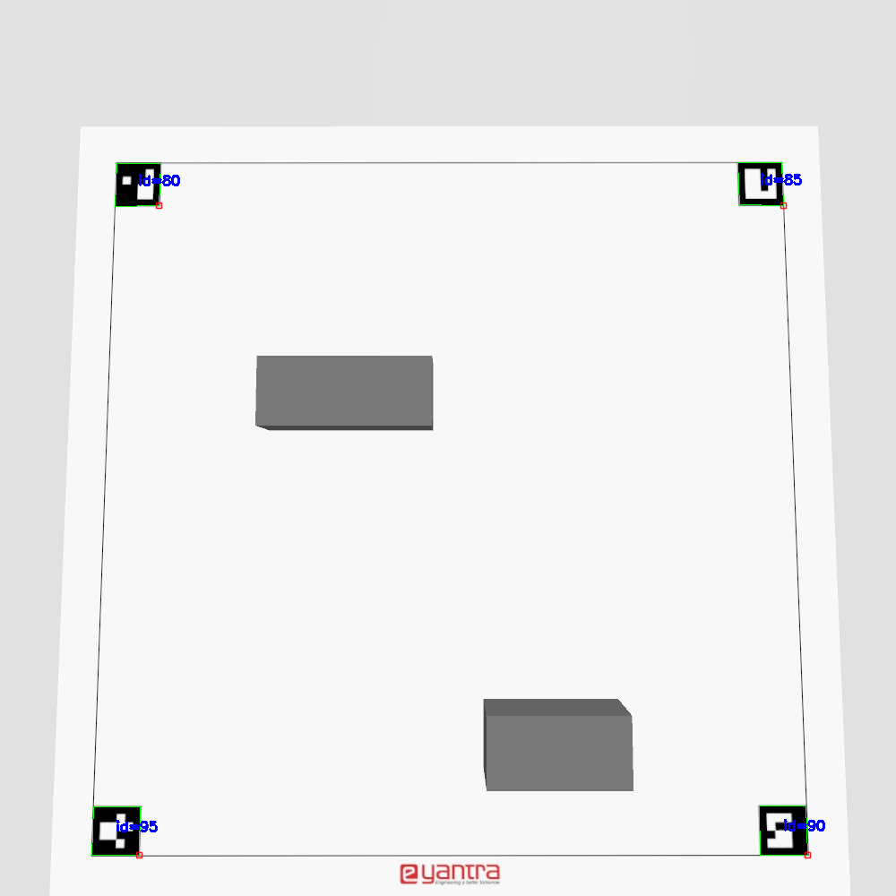
For further visualization, we can draw the markers onto the image using the following code.

detected = aruco.drawDetectedMarkers(frame, corners, ids)
cv2.imshow('detected', detected)

Hence, we get the following image, whcih shows the Aruco markers detected in the image.

---

4. Perspective Transformtion

Once we have detected the Aruco markers, we are able to straigthen out the image and get a proper top-down view of the warehouse.

In technical terms, this is called transforming the perspective of the image. For a perspective transform, we need to know the camera’s focal length, the distance between the camera and the object, and the rotation angle.

However, we do not have this information since our only input is an image. However, we do have the Aruco markers. We obtained the acutal corners of the required image using some simple math as follows:

# Find the respective corners of the Aruco markers
top_lefts = []
top_rights = []
bottom_lefts = []
bottom_rights = []
for corner in corners:
  [top_left, top_right, bottom_right, bottom_left] = corner
  top_lefts.append(top_left)
  top_rights.append(top_right)
  bottom_lefts.append(bottom_left)
  bottom_rights.append(bottom_right)

# Find the innermost corners, whic are the corners of the image
# by using the euclidean distance from the corners of the original image 
# as the sorting key
top_left = sorted(
  top_lefts,
  key = lambda c: c[0] ** 2 + c[1] ** 2
)[0]

top_right = sorted(
  top_rights,
  key = lambda c: (self.width - c[0]) ** 2 + c[1] ** 2
)[0]

bottom_left = sorted(
  bottom_lefts,
  key = lambda c: c[0] ** 2 + (self.height - c[1]) ** 2
)[0]

bottom_right = sorted(
  bottom_rights,
  key = lambda c: (self.width - c[0]) ** 2 + (self.height - c[1]) ** 2
)[0]

Now, using these points obtained from the Aruco markers, we can construct a matrix which encodes all the information required for the transform. We will call this the source matrix. Similarly, we can construct a matrix which encodes the desired transformation. This is called the destination matrix.

src_points = np.array([
  [top_left[0], top_left[1]],
  [top_right[0], top_right[1]], 
  [bottom_right[0], bottom_right[1]], 
  [bottom_left[0], bottom_left[1]]
  ], np.float32
)

dest_points = np.array([
  [0, 0], 
  [self.width, 0], 
  [self.width, self.height], 
  [0, self.height]
  ], np.float32
)

perspective_dest = np.array(dest_points)
perspective_src = np.array(src_points)

Then, using the source and destination matrices, we can calculate a perspective transformation matrix which will transform the source image into the destination image. We pass this matrix to OpenCVs warpPerspective function to apply a perspective transform on the image.

perspective_transform = cv2.getPerspectiveTransform(
  perspective_src,
  perspective_dest
)

transformed_image = cv2.warpPerspective(
  image.copy(), 
  perspective_transform, 
  (self.width, self.height)
)

This process yields an image that looks somewhat like the one below. It appears to be straightened out, i.e. a proper top-down view of what the drone sees.

---

5. Contour Detection

Now that we have correctly transformed our image into a top-down view, we can accurately detect obstacles, and calculate their number and area.

For this, we will use OpenCVs findContours() function. This function is based on the paper Topological Structural Analysis of Digitized Binary Images by Border Following by Satoshi Suzuki and Keiichi Abe. It proposes an algorithm to extract the topological structure of binary images by following the borders of connected components (regions of connected 1-pixels) and holes (regions of connected 0-pixels).

It describes two algorithm as follows.

1. First Algorithm: This algorithm identifies both the outer borders of connected components and the hole borders, mapping out their topological relationships (i.e., which component surrounds which hole).
2. Second Algorithm: A simplified version of the first algorithm, it follows only the outermost borders, ignoring internal holes. This is useful when you want to count only the outer components or simplify the image.

In essence, this paper allows us to detect countours by following the borders where colors appear to change.

We will use the first algorithm t detect image contours (i.e. our obstacles). We’ll also draw these contours onto the transformers image, to visualize how the edges are detected. This is done using the following piece of code.

contours, _ = cv2.findContours(
  transformed_image,
  cv2.RETR_EXTERNAL,
  cv2.CHAIN_APPROX_SIMPLE
)

contoured = cv2.drawContours(
  temp,
  contours,
  -1, (0, 255, 0), 2
)

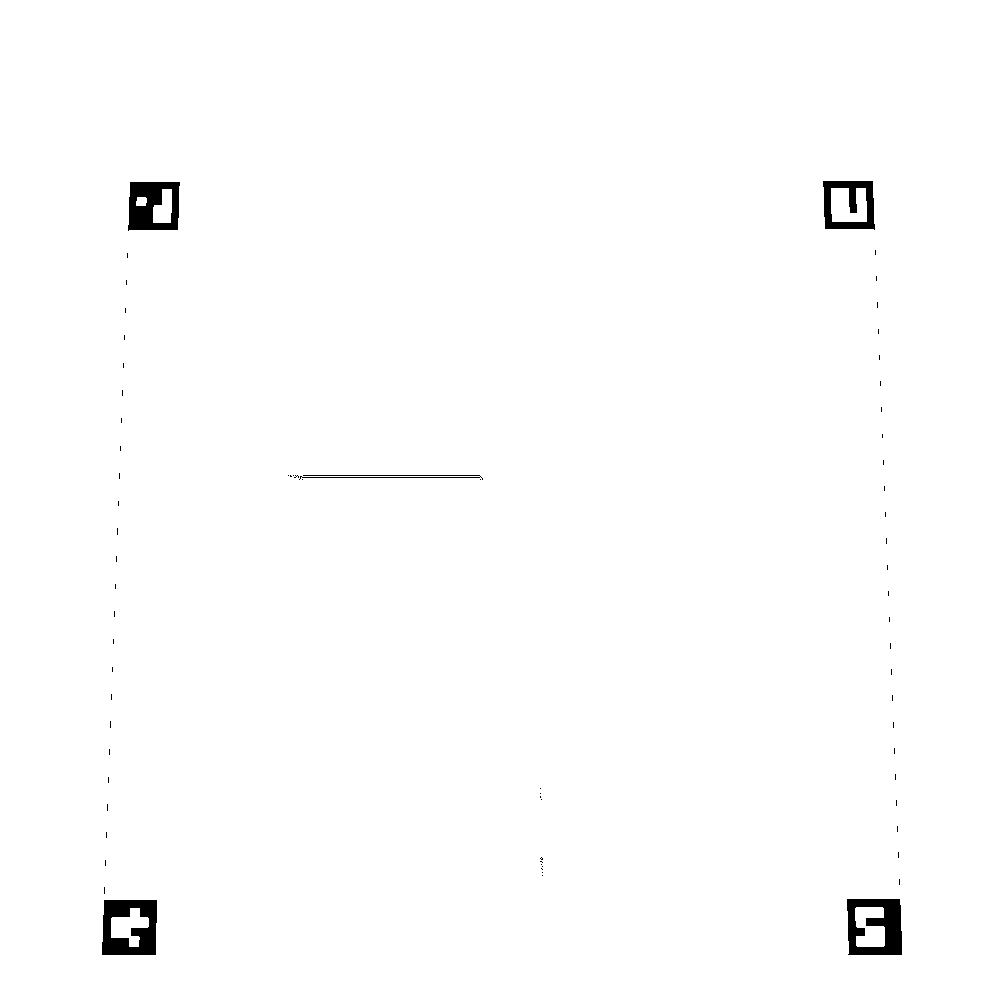
cv2.imshow('contoured', contoured)

The contoured image is shown below.

Finally, we can calculate the total area by using the contourArea() function from OpenCV. Similarly, calculating the number of obstacles is also trivial, as we just count the number of contours with an area that exceeds a particular baseline amount.

total_area = sum(
  cv2.contourArea(contour) for contour in contours
)

min_area = 500  # Adjust this value depending on the size of the objects
filtered_contours = [
  contour for contour in contours 
    if cv2.contourArea(contour) > min_area
]
num_objects = len(filtered_contours)

---

Results

Finally, we were able to calculate the total area of the obstacles in the image, and the number of obstacles.

The results were as follows:

1. Total area = 72141.5
2. No. of obstacles = 2

Our code was also evaluated against multiple other test images (which were inaccessible to us) on the Eyantra evaluation platform. It passed with flying colors securing us 30/30 marks for the task.

---

Conclusion

The image processing techniques utilized in this Python file demonstrate a complete pipeline from Aruco marker detection to obstacle detection and area calculation. Each technique plays a vital role in enabling the detection, transformation, and analysis of the environment:

1. Aruco marker detection is used for reference point detection.
2. Grayscaling simplifies the image by removing color.
3. Binarization converts the image to black-and-white for easier segmentation.
4. Perspective transformation corrects distortions and creates a top-down view.
5. Contour detection identifies objects and calculates their area.

This workflow is particularly useful in robotics and computer vision applications where detecting markers and obstacles in real-world environments is crucial for navigation and analysis.